Pascal's triangle is an arithmetic procedure or algorithm for deriving successive series of what are known to algebra as the binomial series. Whenever approximations to these series appear in data compiled by researchers, they are regarded as showing binomial or random distributions, which mean that they record events happening by chance.
Pascal's triangle of probability distributions graph as discrete approximations to the smooth bell-shaped curve of the normal distribution. This page shows how to graphicly convert Pascal's triangle of binomial distributions into the form of various waves. I could borrow the term probability waves from quantum mechanics. But no attempt is made to explain that here, even if I could. I merely wish to express probabilities in terms of circular motion, which implies wave motion.
The widest known and used pattern of probabilities or frequency table of chance events is given in Pascal's triangle of table 1. This can be expressed formally from the binomial theorem (of Newton).
| 0 | ||||||||||||||
| 0 | 0 | |||||||||||||
| 0 | 1 | 0 | ||||||||||||
| 0 | 1 | 1 | 0 | |||||||||||
| 0 | 1 | 2 | 1 | 0 | ||||||||||
| 0 | 1 | 3 | 3 | 1 | 0 | |||||||||
| 0 | 1 | 4 | 6 | 4 | 1 | 0 | ||||||||
| 0 | 1 | 5 | 10 | 10 | 5 | 1 | 0 | |||||||
| 1 | 6 | 15 | 20 | 15 | 6 | 1 |
Normally, the zeros are not shown in Pascal's triangle, table 1. But the zeros are needed for codifying the triangle's information in graph form. Each row of Pascal's triangle can be put into the form of Cartesian co-ordinates. Each row then can be plotted onto a rectangular graph. When the co-ordinates are joined each row is represented by an angular "curve". Further down the triangle, the rows produce smoother and smoother curves. That would be more evident if these bigger curves are reduced to compare in size to the graphs of the first few rows of Pascal's triangle.
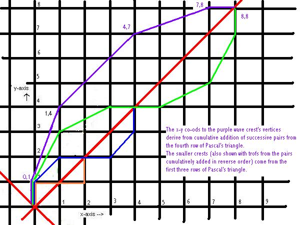
Table 2 shows how the ordered numbers of each row in Pascal's triangle, including the zeros, are successively paired and transformed into co-ordinates by cumulative addition of the pairs. The co-ordinates are then plotted in figure 1.
| Pascal triangle rows | x,y | x,y | x,y | x,y | x,y | x,y | x,y | x,y |
| 1st row pairs: | 01 | 10 | reverse for trof: 10 | 01 | ||||
| 1st row co-ods: | 0,1 | 1,1 | trof co-ods: 2,1 | 2,2 | ||||
| 2nd row pairs: | 01 | 11 | 10 | reverse: 10 | 11 | 01 | ||
| 2nd row co-ods: | 0,1 | 1,2 | 2,2 | trof: 3,2 | 4,3 | 4,4 | ||
| 3rd row pairs: | 01 | 12 | 21 | 10 | reverse: 10 | 21 | 12 | 01 |
| 3rd row co-ods: | 0,1 | 1,3 | 3,4 | 4,4 | trof: 5,4 | 7,5 | 8,7 | 8,8 |
| 4th row pairs: | 01 | 13 | 33 | 31 | 10 | |||
| 4th row co-ods: | 0,1 | 1,4 | 4,7 | 7,8 | 8,8 |
Figure one has the standard x-y co-ordinates. Notice also that a new pair of co-ordinates (in red) at forty five degrees goes right thru the equilibrium points of all the four waves. That is where the crests turn into trofs. This equilibrium line would be zero, or X = 0, from the red X-Y co-ordinate system's point of view.
Measuring the distances between a curve's vertices by the red line (its X ordinate) shows that it conforms to its respective row of Pascal's triangle. That is measured in the units of one half diagonal of a square. The squares are unitary, so the diagonals are the square root of two (by Pythagoras' theorem). Therefore, a half diagonal is (2^1/2)/2 = 1/2^1/2.
This result is confirmed by trigonometry. The red axis, X, is forty five degrees to the black x-axis. The former is a hypotenuse given by x.cos (45 degrees). Thus X = x/2^1/2.
The same reasoning applies to the red Y axis in relation to the black y axis. Thus the Y heights of a curve's vertices from the X-axis are also measures of the terms from a given row of Pascal's triangle, in units of one half diagonal of a square.
Natural philosophers used curves like these as simplified aids to the study of wave motions such as vibrating strings. Thus the vertices would be imagined as the points on a string, where light weights are pulling the string into these crudely wave-like forms. (I attempted to describe this on my page, Coupled oscillator and wave equation.)
So, it is reasonable to suppose that the angular curves in figure 1 may represent progressive approximations to smoothly curved waves. The heights of the curves are given by Pascal rows, which are binomial distributions, and these are not associated with a sine wave. Tho, the usual un-sine-like hump shape of the binomial distribution is changed, in figure 1, because each term is not there separated by an equal distance, but by the same distances as the heights.
Sine waves can be drawn with reference to a circle. Convention takes the upper right quadrant of a circle. A radius line (or vector, having both direction and magnitude) sweeps angles anti-clockwise, starting from the positive x-axis of the circle's quadrature.
Pythagoras' theorem is the equation of a circle: x² + y² = r², where where x and y are the rectilinear co-ordinates that bisect a circle of radius, r. To plot some easy points of the circumference in the upper right quadrant (which is similar to the other three quadrants) label both the x and y axes, in intervals of one-quarter, from zero to one. Draw a straight line from the ends of the positive x and y axes both at unity. This line is like the string to a bow that is a quarter of the full arc of the circle. Take the five x-y co-ordinates: 1,0; 3/4, 1/4; 1/2, 1/2; 1/4, 3/4; 0,1. Take their square roots, respectively: 1,0; (3^1/2)/2, 1/2; 1/(2^1/2), 1/(2^1/2); etc. Plot the latter co-ordinates which form an arc.
The diagonal line, which is the string to the bow, can be re-measured in new co-ordinates by creating an X-Y co-od system at forty-five degrees to the x-y co-ods. Then all the five X-co-ods are: 1/(2^1/2) and all the Y co-ods range from plus to minus this value.
The procedure for turning Pascal rows into Pascal waves is the same as used for graphing the Fibonacci series (as shown on another web page). Pascal's triangle itself can derive the Fibonacci series. Slanting lines are put across the rows to create the new rows shown in table 3.
| Fibonacci series | |||||
| 0 | 1 | 1 | |||
| 0 | 1 | 0 | 1 | ||
| 0 | 1 | 1 | 0 | 2 | |
| 0 | 1 | 2 | 0 | 3 | |
| 0 | 1 | 3 | 1 | 0 | 5 |
| 0 | 1 | 4 | 3 | 0 | 8 |
| 0 | 1 | 5 | 6 | 1 | 13 |
The usual algorithm for the Fibonacci series merely starts with two whole numbers, most simply zero and one. These are summed and the larger of the two original numbers is added to the sum, and so on: 0 + 1 = 1; 1 + 1 = 2; 1 + 2 = 3; 2 + 3 = 5,...
It may be thought this is more self-contained an algorithm, than the above procedure of pairing rows of Pascal's triangle. However, Pascal's triangle itself shows that the number sequence, 1, 2, 3, 4, is not completely elemental. As the outward rows of ones shows, these numbers really represent the operation of adding a unit at a time.
The Pascal-Fibonacci rows, that each sum to a number in the Fibonacci series, can themselves be graphed, producing lop-sided wave forms.
The ratios of successive terms in the Fibonacci series converge to
(1 ± 5^1/2)/2 ~ 1.618 or .618, depending on whether the ratio has the bigger
or smaller value in the numerator.
The Pascal-Fibonacci rows can be averaged, and the ratios of successive row
averages taken. Since the Pascal-Fibonacci series are cumulative series, like
the Fibonacci series itself, a geometric mean would be the suitable average
to use.
Moreover, Pascal's triangle, as rows of binomial distributions, can be varied from symmetrical distributions into skewed distributions. This only requires the binomial theorem to be changed from say, (1/2 + 1/2)^n, where n is any whole number, to an unequal pair of fractions in the factor, say: (2/3 + 1/3)^n. This expands into a skewed distribution.
A skewed distribution, when graphed according to the above procedure, will
produce a skewed wave.
A membrane pushed in at about forty five degrees ( as shown in the Alonso and
Finn text on Physics) looks like a skewed wave, if in two dimensions rather
than one.
Reference.
Martin Gardner: Mathematical Carnival.
Richard Lung.
Written sometime in 2008.
Posted june 2009.