The previous page gave the probable solution for an equation of diffusion or the conduction of heat in one dimension, such as along a rod heated in the middle. The following shows a similar solution for two dimensions ( such as a square metal plate heated in the middle ) by an extension of probability theory.
The diffusion equation in one dimension was of the nature of a random walk back and forth along a line. In the linear case, it is supposed the proverbial drunken sailor leaving the bistro can walk left or right but is not able to decide which. In the two dimensional case, the drunken sailor is supposed to be able to move left or right, back or forth, with equal ease, but not at his own command.
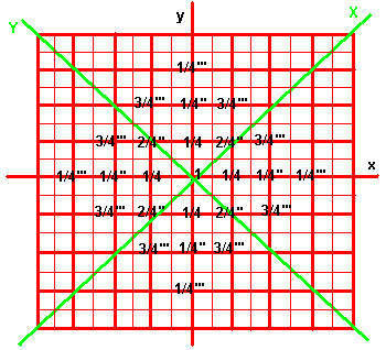
Figure 1 gives a probability map for such random movements. Starting at the center, the probability is one, or a certainty, of being there. For the next step, there are four possible ways to go. This gives each adjacent square a probability of one quarter that will be the next step. ( All the positions are bounded by the thin red lines. )
These and subsequent probabilities are worked out with a difference equation. For instance, to work out any of the four positions, that have one quarter probability of being reached, using the difference equation. The equation works by taking an average of four known probabilities about a central position, whose probability of being reached, is to be found.
If we dont know one of the positions valued at one quarter probability, the difference equation can find it, knowing the probabilities for its four surrounding positions. And we have this information. The position probability to be found is adjacent to the starting position, which has probability one. In one step, it is only possible to move to one of four positions. That means that the probability is zero for arriving at all further positions in that one step.
The two-dimensional difference equation adds the adjacent left and right position probabilities and the adjacent back and forward position probabilities, dividing by four to estimate, as an average, the central position's probability. In terms of this equation, the one-quarter probability positions are averages of one adjacent position having probability one and three adjacent positions having probability zero.
Whatever the second random step to a second position, one or two of its adjacent positions will have one-quarter probabilities. Tho the second random step may move away from the start, the new position occupied still has at least two adjacent positions too far to have been reached and therefore with zero probability of being occupied at that stage.
The probability for a position, with two adjacent quarter probabilities and two adjacent zero probabilities, works out at one quarter of two quarters and two zeros. That is a probability of two-sixteenths. ( The diagram gives the powers as Roman numerals. Thus 2/4'' is the same as 2/4². )
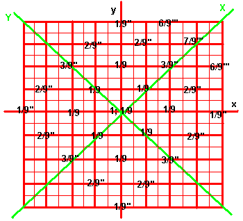
Figure 2 gives the trinomial distribution in two dimensions, compared to figure 1 for the binomial distribution in 2-D. Notice that the first figure is in terms of a 'diffusion' or distribution that takes place one step at a time. But in figure 2, the diffusion is two steps at a time. As before, we start from maximum concentration of probability of one at the center. In figure 1, one step could only reach four adjacent squares, with an equal probability of one-quarter each, for arriving at them randomly. But figure 2 shows there are nine squares that two steps can reach. These are eight surrounding squares and the center square by taking one step out and one step back. Randomly speaking, there is a one-ninth probability of arriving at one of these nine squares.
Moving a stage further in the diffusion or distribution process, how do we arrive, for instance, at the square with the probability estimate of 3/9²? We look at the nine squares that are two steps away from it ( including the square in question, from which we can take one step out and one step back ). We add the probabilities of the previous stage of distribution, that have reached any of those nine squares, and divide by nine. There are three squares of one-ninth probability each within two steps of the square in question. Its probability of being reached in an ongoing diffusion is, therefore, three times one-ninth, divided by nine. That is 3/9².
( The top right corner of figure two shows three of the probabilities for the next distribution stage. )
The two figures show how two distributions, a binomial distribution and a
trinomial distribution, spread in two dimensions. But they dont show, except
for the simplest original distributions, a given distribution state.
From figure 1, the original distribution is concentrated in the center, at one
probability or certainty. The next distribution is four quarter probabilities.
The third distribution state shows a square of eight positions with
probabilities of either one or two sixteenths. They add up to twelve
sixteenths. The remaining four sixteenths are to be found in the center,
because the four one-quarter probabilities are each one step away from the
center, as well as the eight outer adjacent squares. This completes the
probability distribution for the third stage of diffusion.
Similar considerations apply, in figure 2, for a given stage of the trinomial distribution. For the third stage, the denominator of the probabilities is nine squared or eighty one. This means that there must be enough squares found, for this distribution, so that the numerators add up to eighty one, conserving the initial distribution concentrated in the center at a value of unity.
Figure 2, like figure 1, shows a distribution in process, not the state of, say, the third distribution. Counting the numerators, of all the squares shown with denominators of nine squared, they only add up to 32 out of 81. That partial sum comes from stepping out from eight squares each of one ninth probability. But those eight positions can also take two steps into their neighbors' positions. The four corner positions each add up to probabilities of 4/81. And their four inter-mediate positions each add up to 6/81. This adds four times four equals sixteen and four times six equals twenty four. This forty on top of thirty two gives 72 out of 81. The final nine out of 81 comes from the central position which can be reached in two steps by the square of eight and by itself, making nine times one-ninth, divided by one-ninth.
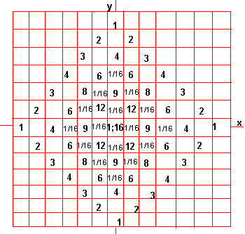
Instead of having to imagine this, figure 3 shows just this stage, we have been describing for the third stage of the trinomial distribution, for the third stage of what comes after the binomial and trinomial distributions. The binomial distribution was based on two equal probabilities, in two dimensions, resulting in one half of one half or one quarter probability for the next one of four steps. The trinomial distribution considered three one-third probabilities in two dimensions, resulting in nine possible two-steps of one-ninth probability each.
The distributions coming after the binomial distribution are examples of the multinomial distribution, starting with the trinomial distribution. Next is the possibility of four one-quarter probabilities, or a 'four-nomial' distribution. In two dimensions, this involves the square of one-quarter, or one-sixteenth probabilities.
Thus, figure 3 is based on sixteen squares each of one-sixteenth probability of being reached in three steps from the central position, which, as usual, has the initial concentrated distribution of one out of one probability. This 1 is shown in the central square. All the other whole numbers, including the 16 in the same square are actually out of 256, or sixteen squared, which is their sum.
Notice that the border or boundary numbers on two adjacent sides form a multiplication table for the value of an interior square they co-ordinate. Thus, the central value of 16 is cross-referenced by any two adjacent boundary sides, whose values are both four: four times four equals sixteen. But that number sixteen was found because it takes three steps to reach from each of the sixteen squares marked at one-sixteenth. In the case of the inner four positions, adjacent the center, the three steps mean one step forward one step back and one step forward again into the center. ( This describes the four-nomial entry in table one, below. )
Further stages of the ( uniform ) multinomial distribution use five fifths, six sixths, seven sevenths etc. See table one to help map these distributions in two dimensions. Tho, for all practical purposes, the immense number of arithmetic calculations in finite difference equations have been the work of computers since their beginnings.
| Constants | Steps per move | 0 to 3 retraced steps per move nest positions | |||
|---|---|---|---|---|---|
| 0 | 1 | 2 | 3 | ||
| 1/1 | 0 | 0 | |||
| 1/4 (binomial) | 1 | 4 | |||
| 1/9 (trinomial) | 2 | 8 | 1 | ||
| 1/16 (four-nomial) | 3 | 12 | 4 | ||
| 1/25 | 4 | 16 | 8 | 1 | |
| 1/36 | 5 | 20 | 16 | ||
| 1/49 | 6 | 24 | 16 | 8 | 1 |
The above example of a multinomial distribution in two dimensions simply extends to a three-dimensional distribution. Take the axes of the two dimensions at 45 degrees to the x-y axes shown in figure 3. ( That is the axes shown in green in fgures 1 and 2. ) A third axis would be perpendicular to the plane, turning it into a cube, with the same values, at the edge, as those for the edges of the plane.
That is 1, 2, 3, 4, 3, 2, 1 for a third or z-axis, as well as the x and y axes. Considered as fractions of only 16, this series is the complete multinomial distribution in one dimension of
( 1/4 + 1/4 + 1/4 + 1/4 )².
To see how this can be, the four quarters each may be labeled a, b, c, d, or made coefficients of a = b = c = d = 1. Expanding the square of the four quarters then shows that the one 4, in the boundary values, corresponds to one set of 4 values that are the squares of a, b, c and d. A four-by-four table of the sixteen combinations of the expansion may show the four letters squared in diagonal position. There are two adjacent diagonals of three combinations each. Next adjacent are two diagonals of two combinations and finally one combination each are at diagonally opposite corners of the square table. These pairs of 3, 2 and 1 diagonals have all their letter combinations reversed to each other. See table two.
| aa | ab | ac | ad |
| ba | bb | bc | bd |
| ca | cb | cc | cd |
| da | db | dc | dd |
Consider the edges of a cube with boundary values that are those of a one-dimensional ( multinomial ) distribution. As every ( one-dimensional ) edge of the cube has the same boundary values, every face of the cube has the same values as the ( two-dimensional ) plane of figure 3. The probability density of the cube is greatest at the center, co-ordinated by three axes each of value 4, to give it a probability of 4³ out of (16)³.
Logicly, distributions could be carried into higher dimensions than the three dimensions of space that our senses recognise. Probability distributions could spread into a hyper-cube of four or more dimensions. We might not be able to imagine what a four-dimensional hyper-cube looks like. But it is simple enough to consider the abstract proposition.
The example above was of a cube with three dimensions of possibilities that summed to (16)³. In one higher dimension ( hidden to our senses ) the number of possibilities becomes sixteen to the power of four. The densest probability, at the center, was 4³ for the cube. For the 4-D hyper-cube, this becomes four to the power of four.
So far, only perfectly regular distributions have been considered, based on equal probabilities of stepping in one direction or another. The binomial distribution in one dimension gives a half and half probability of moving one way or another in a straight line. In two dimensions this becomes a quarter probability of moving left-right or back-forward. The trinomial distribution in one dimension offers three equal possibilities of one-third for moving in a straight line, and nine possibilities each of one-ninth for moving in two dimensions.
The multinomial distribution for four equal possibilities of one-fourth, in one dimension, becomes sixteen equal possibilities of one-sixteenth in two dimensions.
Suppose the possibilities for movement are not equal but skewed, resulting in a skewed distribution. Suppose the drunken sailor carries a kit bag over his left shoulder that makes him twice as likely to move to the left than the right in his still otherwise random motion one way or the other. In other words, suppose we change the regular binomial distribution in one dimension with its probabilities of one half one way and one half the other, and make those probabilities two-thirds to the left and one-third to the right.
In two dimensions, the probabilities would be out of six, rather than three, because one step to the east and two steps to the north must have a corresponding one step to the west and two steps to the south, totalling six. From these initial conditions a probability table can be built up, similarly to figures 1 and 2, except that the distribution will be systematicly skewed, because the probabilities will always be doubled to north and south, whereas to east and west probabilities are merely added as in figures 1 and 2. See figure 4.
| 8/216 | ||||||
| 12/216 | 4/36 | 12/216 | ||||
| 6/216 | 4/36 | 2/6 | 4/36 | 6/216 | ||
| 1/216 | 1/36 | 1/6 | 1 | 1/6 | 1/36 | 1/216 |
| 6/216 | 4/36 | 2/6 | 4/36 | 6/216 | ||
| 12/216 | 4/36 | 12/216 | ||||
| 8/216 |
Looking at figures 1 and 2, the dynamic of diffusion depends on successive divisions by four and nine, respectively, for each successive distribution. This particular skewed distribution comes somewhere in between, depending on successive divisions by six.
Notice how the skewing rule applies for transforming one stage into the next. There are six squares of probability value 4/36. First take the four that are adjacent to both 2/6 and 1/6. In these four cases, the value 2/6 is adjacent only to the east or west. In this example, east or west values contribute without weighting.
The other value of 1/6 is always north or south. The skew rule, in this example, says such adjacent values always make a doubled contribution. That is twice one-sixth. Hence the total contribution is 2/6 plus twice 1/6, which comes to four-sixth. Dividing 4/6 by six gives the required value of 4/36, shown in the table.
Now take the remaining two values of 4/36 in the mid column ( actually the y-axis ). The only contributing probabilities, from the previous distribution stage, are 2/6. But since these sole adjacent contributing squares are to the north or south, the skew rule says double 2/6, which gives 4/6. This is divided by six to give 4/36 again.
Having shown the dynamic of the skewed distribution, a whole skewed distribution state, the fourth stage, is shown in figure 5.
| 8/216 | ||||||
| 12/216 | 4/36 | 12/216 | ||||
| 6/216 | 4/36 | 36/216 | 4/36 | 6/216 | ||
| 1/216 | 1/36 | 27/216 | 10/36 | 27/216 | 1/36 | 1/216 |
| 6/216 | 4/36 | 36/216 | 4/36 | 6/216 | ||
| 12/216 | 4/36 | 12/216 | ||||
| 8/216 |
The same skew rule applies to figure 5 of a static distribution. First of all, it should be explained that in figure 4, only 26 out of 36 possibilities are showing. The remaining 10/36 are to be found in the center ( as shown in figure 5 ). As figure 4 shows, the center has 2/6 to the north and 2/6 to the south. The skew rule says double them both, which comes to eight. Then there are two contributions east and west, of 1/6 each, bringing the total to ten. This ten sixths is then divided by six, to give the value of 10/36.
That gives us the necessary full complement of 36 out of 36 possibilities, in their locations of a skewed distribution, to determine the next stage of their diffusion, in terms of 216 out of 216 possibilities. These are all shown in figure 5.
On the previous page, the form of the diffusion equation was shown in one spatial dimension. The two dimensional version is not much different. Formerly, ih represented the spatial dimension, where i = 1, 2, 3,.. and h is a constant, say the x ordinate. In two dimensions, the y ordinate, gh, may stand for a comparable second dimension. The simple case of the same constant, h, is assumed and g is like i, except at ninety degrees, for the second dimension of space. This is in keeping with the above figures which show the two spatial dimensions, the x and y co-ordinates, squarely symmetrical to each other.
As with the spatially one dimensional equation, the two dimensional diffusion equation also has one dimension of time. The diffusion equation is characterised by a first order change in diffusion, or the process of distribution, with respect to time, on one side of the equation, and, on the other side, a second order change of distribution with respect to space, in one or more dimensions.
Comparing how the 1-D equation was reached, the form of the 2-D equation might be rendered as follows, assuming that the constants k/h² = 1/4. ( In the equation, below, the symbols that text-books usually write as subscripts are preceded by commas. )
U,i,g,j+1 - U,i,g,j = 1/4{ U,i+1,g,j - 2U,i,g,j + U,i-1,g,j
+ U,i,g+1,j - 2U,i,g,j + U,i,g-1,j }.
The 1-D equation reduced to simpler form ( known as Schmidt's method ) when k/h² = 1/2. This 2-D version reduces for the value of 1/4:
U,i,g,j+1 = 1/4{ U,i+1,g,j + U,i-1,g,j + U,i,g+1,j + U,i,g-1,j }.
This difference equation symbolises the repeated arithmetic operations that built up the binomial distribution in two dimensions. Suppose the solution of the equation, on the left side, is 2/16, which appears four times in each of the four quadrants of figure 1. Depending on which quadrant is refered to, two of the four terms, on the equation's right side, have values of U equal to one-quarter. There is a diffusion, from unitary probability at the center of figure 1, to two squares, in a given quadrant, beside the square whose probability of being reached is to be estimated from them.
The remaining two adjacent squares, in each quadrant, that come after the probability square in question, are too many steps away to have yet been reached and assigned other than zero probability of arrival so far.
On the left side of the equation, the x and y axes are related to i and g, respectively. On the right side, i and g are always marked either plus one or minus one. This means moving one step on the x or y axes in either a positive or negative direction. In terms of this example, the above equation for 2/16, in the first quadrant, would be written: 2/16 = 1/4{ 0 + 1/4 + 0 + 1/4 }.
Re-label this simplified diffusion equation as: B = 1/4( A + C + D + E ). Re-write it: ( C - 2B + A ) + ( D - 2B + E ) = 0. That is two second order changes of distribution, with respect to space, cancel each other. In terms of the example: ( 1/4 - 2.2/16 + 0 ) + ( 0 - 2.2/16 + 1/4 ) = 0.
This is essentially a form in simple arithmetic ( or the finite difference equation ) corresponding to Laplace's equation. This is another standard partial differential equation related to the diffusion equation. Text-books commonly show Laplace's equation in two dimensions. ( Of course, it can be in other dimensions. ) The diffusion equation in two dimensions reduces to Laplace's equation when the dependent variable, such as a probability distribution, does not change with respect to time.
Figures 1 and 2, for instance, especially if turned 45 degrees in accord with the green axes, respectively show an advance of the binomial distribution ( Pascal's triangle ) and the trinomial distribution, in each quadrant. The numerators of the two dimensional probabilities are the same as for one-dimension. But their squared denominators reflect the greater spread of probabilities over two dimensions. Hence the change, between the one dimensional cases and the two-dimensional cases of the difference equation, of constants of 1/2, 1/3, etc: They are squared to 1/4, 1/9 etc, in the transition from a straight line to a square -- if you like, from a lane to a field.
Further source:
Carl-Erik Froberg. Introduction to Numerical Analysis. 2nd edition 1969.
Richard Lung
3 december 2003