 (Tpi/2)
Section links:
A functional relation between two varying factors may be expressed as an equation. This assumes a definite one-to-one relationship, however elaborate, at all stages being considered. The equation may be drawn as a curve on a graph, whose axes are the two related variables. But the terms of the equation may be difficult to work out algebraically. Sometimes the function may be expanded as an orderly series of terms that systematically approximate the relation.
The simplest and most approximate of such a series is the graph of a straight line, y = a + bx. The constant, a, determines at what height the line passes thru the vertical y-axis. If a = 0, the line passes thru the origin. The constant, b, determines the slant of the line. If b = 1, then y = x, and the line passes thru the origin equidistant from the y- and x-axes.
The point is that by choosing suitable values for the constants, the line can be placed anywhere on the graph. If necessary, a series of straight lines can be drawn to produce an angular approximation to a curve. For instance, the more sides drawn to a regular polygon, the closer it comes to the curve called a circle.
Thus, a line ( such as the side of a polygon ) passes thru two points on a curve ( such as a circle ). The method of simultaneous equations is used to solve the values of their constants. It takes two equations of a straight line, both with the same constants, a and b, to solve them if they are unknowns.
Similarly, for the next step up in equations, from straight lines. That is
a series equation with an extra term to one higher power, and with one extra
constant, namely cx². This is the equation of the curve called a parabola. Its
three constants may be adjusted to approximate, in three places the curve of
some function we are interested in. This is instead of just two matches by the
straight line.
It takes three simultaneous equations, containing a, b and c, to solve them as
unknowns.
The next step up in a power series is the cubic equation, with a cubic
power of x, and a fourth constant coefficient, d. That is dx³.
The above three power series are sometimes called polynomial equations of the
first, second and third degrees, respectively equations of straight lines,
quadratic equations ( of parabolas ) and cubic equations. The fourth degree
equation adds a further term, to the fourth power of x, multiplied by a fifth
constant.
The higher the degree of the polynomial the more points at which some function may be represented within a range however long. This does not always work but many functions can be expanded in power series. The path of the power series is found by evaluating the constant coefficients of its terms, by a method of successive differentiation.
Differentiation, as in the fearsomely named differential calculus, is basically a clever bit of algebra, known as differentiation from first principles. Its best known example is that the differentiation of distance traveled, with respect to time, derives the velocity. In other words, the velocity is the 'derivative' of distance with respect to time ( in a given direction ).
Suppose a distance, x, in metres traveled after a time, t, in seconds, is always the square of the time. So, after one second, the distance traveled is one metre. After two seconds, the distance traveled is four metres; after three seconds, nine metres, and so on. This can be expressed as the formula x = t².
Differentiation of this equation gives another equation, for the velocity, v ( or speed in a given direction ) after t seconds. Differentiations of equations from first principles often follow patterns, so it may be known by rule what is the derivative of x re t. Differentiation is historically expressed in more than one notation, such as dx/dt or x'. If x = t², x' = v = 2t.
In terms of our example, this means after one second the velocity is twice one, or, two metres per second. After two seconds, the speed in a given direction is twice two, or, four metres per second; after three seconds, the speed is six metres per second, and so on. The velocity shows the rate of change of distance with respect to time.
Differentiation from first principles gets this result as follows. From x = t², we add a small change in the distance, ^x, to distance x, as a result of a small change in the time, ^t, added to time, t. The terms of the equation produce the following:
x + ^x = ( t + ^t )².
To isolate the effect of change of time on change in distance:
x + ^x - x = ( t + ^t )² - t².
Therefore, ^x = 2t^t + (^t)².
Therefore the ratio of change of distance to change of time is:
^x/^t = 2t + ^t.
As the change in time gets smaller, so that the change in time approaches a limit of zero ( lim ^t --> 0 ), then the value 2t, given above, is derived.
Differential calculus is about relations considered in these terms of continuous changes taken to their limits. But this is approximated by a 'cruder' calculus of finite differences, that takes ratios of discrete measures.
From the example of x = t², it is known that after one second, an object traveled one metre. After two seconds, the object had traveled four metres. That is three metres were traveled in the second second. So, after one second, the speed is somewhere between one and three metres per second.
Such rules are only a true measure of a changing reality, in so far as everything is happening as smoothly in practise. This is one of the basic qualifications for calculus to apply. Assuming this is so, x = t² applies also to fractions of time and distance units. So, after .9 seconds, the distance is .81 metres. In the tenth of a second between .9 and 1 second, the object goes .19 metres. This gives an average speed of .19/.1 = 1.9 metres per second.
Similarly, after 1.1 seconds, the distance is 1.21 metres, for an average speed of .21/.1 = 2.1 metres per second. Taking differences of a thousandth of a second, the average speed works out at between 1.999 and 2.001 metres per second.
Thus a finer calculus of finite difference ratios approximates the ultimate ratio provided by differential calculus, in this case, the velocity ( or speed in a given direction ) of 2t for t = 1. Calculating similar finite differences of distance over time, for just before and after the second second would approximate a velocity of 2t for t = 2, or four metres per second.
In the above example, the differentiation rule saved a lot of arithmetic by finite differences. But the rules often cannot be found. And with increasingly powerful computers, it is often easier to solve dynamic problems with programs for all the ghastly arithmetic involved in the calculating of finite differences.
The velocity, in its turn, has its own derivative, called the acceleration,
a. In the example, the acceleration is represented by the feature that the
velocity is always twice the number of seconds. The acceleration is constant
at two metres per second per second.
Using the notation, x'' = v' = a = 2.
In this example, successive differentiation has successively reduced the independent variable, the time. And in fact, the rule for differentiation of a constant, such as two, is to reduce it to zero. In other words, the acceleration does not, in turn, have a rate of change of its own. The rate of change of the acceleration, with respect to time, is zero. Had we started with a relationship between distance and time, involving a higher power of the time, then acceleration would have had a rate of change not yet reduced to nothing.
However, successive differentiation may eventually eliminate terms in polynomial equations, so that the constant, in the remaining term, may be isolated and determined. ( We must know where we are with a series to derive sensible results from it. Generally, we are talking about so-called convergent series, meaning an orderly arrangement of successive terms that may be of indefinite length but still approaches a definite sum. )
Take two variable factors, u and x, where u is determined by x, or u is a function of x, symbolised by u(x). Suppose this function can be expanded by a power series ( where the comma, after constant, a, means that the following numbers 0, 1, 2, 3, etc are only notation -- texts usually put in subscript -- for the zeroth, first, second, third etc constants ) so:
u(x) = a,0 + a,1x + a,2x² + a,3x³ + ...
The first order differentiation of u(x) is:
u'(x) = a,1 + 2a,2x + 3a,3x² + ( 4a,4x³ ) + ...
The second order differentiation is:
u''(x) = 2a,2 + 3.2a,3x + ( 4.3a,4x² ) + ... = 2a,2 + 6a,3x + ( 12a,4x² ) + ...
The third order differentiation is:
u'''(x) = 6a,3 + ( 24a,4x ) + ...
The fourth order differentiation is:
u''''(x) = 0 + ( 24a,4 ) + ...
Values for the constants, in the successive terms, can be found for when x = 0, in relation to the derivative values of u. These constants give the points at which the derivatives of u, considered as curves, cross the vertical axis, where the horizontal x-axis is zero. Thus:
u(x) = u(0) = a,0.
u'(x) = u'(0) = a,1.
u''(x) = u''(0) = 2a,2 = 2!a,2.
u'''(x) = u'''(0) = 6a,3 = 3!a,3.
u''''(x) = u''''(0) = 24a,4 = 4!a,4.
( The apostrophes symbolise a factorial number, which multiplies itself by
all its lesser whole numbers. Thus 4! = 4.3.2.1. )
Substitute these values for the constant coefficients in the power series:
u(x) = u(0) + u'(0)x + u''(0)x²/2! + u'''(0)x³/3! + ...
This is called Maclaurin's series for the function u(x).
One, of mathematics' two most important constants, is the exponent ( shortened
to exp or e ) which is an infinite number 2.718... The function exp(x), or the
exponent to the power of x, has the special significance that it remains the
same under successive differentiation. Using the example of distance traveled
over time, this function would show distance increase geometrically with each
unit of time. Taking the derivative of distance with respect to time, for the
rate of change of distance with respect to time, or the velocity, shows
exactly the same geometric increase. Similarly, the acceleration, or change of
velocity with respect to time, is the same geometric increase. Exponential
change is constancy in orders of the rate of change. ( There is exponential
decrease or decay as well as increase. )
Thus, exp(x) = exp'(x) = exp''(x) = exp'''(x) = ...
It so happens that when x = 0, the exponent of x equals one: exp(x) = exp(0) = 1. Therefore all the successive derivatives of the exponent of x also equal one. Substituting these ones into Maclaurin's series for the exponential function means that it can be computed by adding this series of terms:
exp(x) = 1 + x + x²/2! + x³/3! + ...
Note, the exponent itself, that is the exponent to the power of x equals one, can be calculated as a numerical series that approaches an infinite number beginning 2.718...
The same method finds the series, for example, of the binomial function and the trigonometric functions.
Maclaurin's series is a special case of Taylor's series, which can be shown with the help of figure one. Take the vertical axis for u(x) to be the dashed line. Then the position, underneath it, x is at zero. The derivative terms that make up Maclaurin's series express the function u(x) at the point A, above x = 0.
Moving the distance, h, to the right of x, Maclaurin's series expresses, at point B on the curve, a function u(h), instead of u(x). The only difference in the series is that letters x are replaced by letters h.
Figure one shows the u(x) axis moved distance, a, to the left. At point A, the curve becomes a function of a, instead of x = 0. At point B, the curve is a function of (a+h). If x = a, then Maclaurin's series may be generalised from a function of u(x) to a function of u(x+h) called Taylor's series:
u(x+h) = u(x) + u'(x)h + u''(x)h²/2! + u'''(x)h³/3! + ...
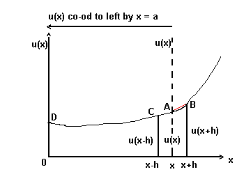
This function is shown on figure one, as is u(x-h) which expands as:
u(x-h) = u(x) - u'(x)h + u''(x)h²/2! - u'''(x)h³/3! + ...
As discussed, finite differences can approximate derivatives. By subtracting u(x-h) from u(x+h), a finite difference approximation of the first derivative may be obtained, assuming higher powers than h² are negligible enough to be ignored:
u'(x) ~ { u(x+h) - u(x-h) }/2h.
In figure one, this equation represents the slope of the chord CB. As a first order finite difference equation, it approximates the derivative, which would be geometrically represented by a tangent to the curve at point A.
This formula for u'(x) is called a central difference approximation, because two other approximations are also possible. The forward-difference formula is represented by the slope of the chord AB ( shown in red in figure one ):
u'(x) ~ { u(x+h) - u(x) }/h.
( There is also a backward-difference approximation to u'(x) for the slope of the chord CA. )
The second order finite difference approximation to a second derivative can be obtained by adding the two versions of the Taylor's series, this time ignoring as negligible all fourth or higher powers of h:
u(x+h) + u(x-h) ~ 2u(x) + u''(x)h².
Therefore,
u''(x) ~ { u(x+h) - 2u(x) + u(x-h) }/h².
Many problems in classical physics were solved with second order differential equations. That is equations containing no higher order than a second derivative. Some are called ordinary differential equations, because one factor is determined by only one other factor. That is the dependent variable has only one independent variable, as in the simple example given of distance as a function of time.
Partial differential equations have one dependent variable and two or more independent variables. For instance, a particle may be displaced over time, which is one independent variable, and over space, along one, two or three dimensions, which constitute up to three more independent variables.
Partial differential equations have three standard mathematical forms of widespread application. Finite difference equations can approximate them using the above approximations for first and second derivatives.
To show how this is done, take the example of the diffusion equation ( or heat conduction equation: same form, different application ) in finite difference form. This equation factors, say, concentration of particles in a fluid, over time and space ( most simply in one dimension ). Or, the conduction of heat depends on one spatial variable for heat dissipation along a one-dimensional bar, as well as dissipating in time, a second independent variable.
This form of partial differential equation ( called a parabolic equation ) has various notations. My keyboard allows U'(T) = KU''(X). This says that the first derivative of a factor U, with respect to time, equals a constant K, multiplied by the second derivative of the factor, with respect to one dimension of space, X.
A constant in an equation tends to apply to one physical situation. Getting rid of the constant leaves the mathematical form for every physical situation to which it may apply. There is a proper procedure for this. But it turns out that another time t can be set equal to KT. So:
u'(t) = u''(x).
There x =X ( assuming, in the heat conduction equation, a unit length of rod ). And u = U/U,o. U is the temperature at a distance X from one end of a thin rod after a time T. U,o is, say, the maximum or minimum temperature at zero time.
Figure one shows the finite difference function u(x) in elevation. The curve might be a slide seen from the side. But seen from above, that is in plan, the slide would look like the one dimension of space that is line x. When u is a function of two variables, these two dimensions may be represented in rectangular co-ordinates. Moving from one to two dimensions is like moving from a lane to a field or a line to a rectangle.
Figure two shows the grid plan of the diffusion equation as a finite difference equation.
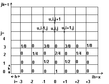
This difference equation sets the distance variable, x, as equal to ih, where h is the length of one grid unit and i is the number of these grid units ( i = 0, 1, 2, 3,.. ).
Thus: u''(x) ~ { u(x+h) - 2u(x) + u(x-h) }/h² becomes { u,i+1,j - 2u,i,j + u,i-1,j }/h².
The j letters have entered the formula, because j ( = 0, 1, 2, 3,.. )
counts the number of grid units for time on the other ordinate. Unlike i in
this formula, j is not adding or subtracting grid units, because this is the
spatial dimension, in which time is held constant.
( Note that the use of commas, before the grid notation i and j, replaces
their usual placement as subscripts in mathematical texts. )
Coming to the time dimension, the grid units have a length of time, k. So, t = jk. For the first order derivative of u with respect to time, it is usual to take the forward-difference formula ( because it is convenient to use in the finite difference equation of diffusion ).
Thus: u'(x) ~ { u(x+h) - u(x) }/h as a first order ordinary finite
difference in space becomes { u,i,j+1 - u,i,j }/k as the first order partial
difference in time.
Note on this occasion, it is the space units, i, which remain unchanged,
because the spatial variable is held constant in the time dimension.
Equating finite temporal and spatial halves of the diffusion equation:
{ u,i,j+1 - u,i,j }/k = { u,i+1,j - 2u,i,j + u,i-1,j }/h².
If the ratio of the constants, k/h² is one half, then the finite difference equation simplifies to:
u,i,j+1 = { u,i-1,j + u,i+1,j }/2.
In figure two, an example, of the relative positions of the three terms of this equation, is shown on the grid. The equation's left-hand term is the unknown, positioned on the grid above the equation's two right hand terms, positioned diagonally below it, on the grid. The latter two terms are the knowns, which, in solving the unknown term, solve the equation.
An arithmetic example, of how this finite difference solution of the diffusion equation works, is also shown on the grid. For any equation to be solved in terms of a particular result or specific output, then a specific input, say of spatial and temporal values, must be fed into the equation. The jargon for these is the boundary conditions and initial conditions.
In the example illustrated, the conditions are k/h² = 1/2. Also, at the initial time, when j = 0, only the mid-point, at unit value, has more than zero value. The two known terms are separated by one grid unit. Taking one of them as the mid-point on the bottom row of the grid, this is added to the value, either two points to the left or the right. Both values are zero, so the result will be the same, in fact a symmetrical distribution will ensue.
This turns out to be the binomial distribution. For, using the finite difference equation, one plus zero, then divided by two, equals one half, on the grid's second row up, when j = 1 and time moves on by t = jk units. On the second row, 1/2 is both to the right and left, of 1 on the bottom row.
The distribution that this finite differnce equation is building up, is simply the way that Pascal's triangle is constructed. It may not be immediately obvious because Pascal's triangle is usually drawn with just the numerators of the numbers shown on the grid. But the denominators, also derived on the grid, are just the sums of the numbers in any row of Pascal's triangle. That is to say that as the input of the equation is one unit at the start, that unitary value is conserved thru the succeeding stages in time, tho it is increasingly dispersed into smaller and smaller fractions.
This process simulates the middle of a rod being heated and the heat being conducted away, over time, symmetrically both ways along a uniform rod. Similarly, for the diffusion of particles in a fluid.
Working with finite difference equations can produce unreliable or unstable results, under certain conditions. For the diffusion equation, the results become unstable when k/h² is greater than one half.
That assumes that the diffusion equation's constant, K, equals one. For,
more generally, the upper limit of one-half applies to Kk/h². So, K could be
set at a half and k made one. Then both sides of the grid mesh would be in
units of one.
Having said, above, that t = KT, that means the diffusion equation would now
be expressed in terms of T for time, with K as its coefficient.
In finite mathematics or statistics, there is a formula for deriving the terms of the binomial distribution, without the need to go thru the sequential process of the finite difference equation. Describing it as a function U:
U = {p'(N-X).q'X}N!/X!(N-X)!
This gives the probability as a fraction of total probability or certainty, one.
N stands for the largest value of X, which can be any whole number from 0
to N. ( Note that a single quotation mark signifies "to the power of". )
The function is a probability function, in which U states a probability with a
given a position and time. A complete probability is defined as the sum total,
or unity, of probabilities and is conventionally set at one. The values p and
q are relative probabilities, such that one or the other must happen, and
therefore must total unity.
The binomial distribution is symmetrical, because the relative probabilities are equal, that is p = q = 1/2.
This simplifies the probability formula to:
U = { (1/2)'N }N!/X!(N-X)!
In the case of heat conduction in a uniform bar, the heat energising of the molecules in the middle of the bar will activate random collisions along both sides of the bar. On aggregate, these collisions will be of roughly the same magnitude and gradually subside in about the same way.
If the bar were not uniform, so that its conductivity differed from one side to the other, then this asymmetry would be modeled by some sort of skewed distribution. The greater to lesser probabilities of heat conduction, on one side to the other, might be estimated at, say, 2/3 to 1/3.
Going back to the symmetric binomial distribution, take an example from figure two. T = jk = j ( if k = 1, for T ). Consider T = j = 3. Also X =ih = i. Consider X = 1.
( Note, this ignores the negative values of X shown on figure two. On the grid, X has twice as many steps -- each at half the length -- as X in the binomial probability formula, which would make it twice the number. But X on the grid has been divided into positive and negative numbers. So, positive X on the grid coincides in its number range with the formula X.
In an illustration, given below, of the 'diffusion' of seats per
constituency in a varyingly multi-member system, the number of seats per
constituency is given by X in the formula. X on the grid would be the
variation, from the average number of seats, given in plus or minus
half-seats, where the half-seats are conveniently treated as units.
If X on the grid were halved, so that the variation was in whole seats, then
the odd-numbered rows of Pascal's triangle, that do not have one actual
average constituency distribution, have to be measured, explicitly, in a
positive or negative half-seat variation from the middle of the two largest
distributions closest to average. The next variation from average is at plus
or minus one and a half seats, followed by two and a half seats, and so on.
)
Continuing the probability formula example, the result is that U is 3/8, for the probability, at that time and place, of concentration of a solution or heat conduction level. That is from having diffused or conducted from an initial time and place of total probability, one, of finding the initial concentration.
Put the above example's values for X and N in the binomial probability formula:
{(1/2)'3 }3!/(3-1)!1! = (1/8)6/2 = 3/8.
Multiplying, by (1/2)'N = (1/2)'3 = 8, would give a probability of 3 out of 8 chances, instead of 3/8 of ( the certainty of ) one.
This formula solution of a finite difference equation of diffusion has its equivalent solution of the differential equation of a continuous function of U with respect to X and T:
U(X,T) = exp{-(±X)²/2T}/(Tpi/2)
If X is made equal to zero ( which yields the modal value of the binomial
distribution for U ) then the exponential term reduces to one. The remaining
term, 1/(Tpi/2) can be shown to be equal to the
binomial probability formula, for X = 0, which is:
N!/{(N/2)!(N/2)!} Then substitute the factorial numbers for Stirling's approximation.
Namely, N! ~ N'N.exp(-N)(2piN)
( where N'N means N to the power of N. And where pi stands for the Greek letter of that name ).
The relative size of the error in Stirling's approximation reduces for larger
numbers.
For N = 6, the binomial formula gives the mode of the binomial distribution as 20 ( after dividing by (1/2)'N = 1/64. ) The differential equation solution gives about 20.84 ( after multiplying by 64 ) for the mode of the normal distribution, the continuous bell-shaped curve compared to the binomial distribution's stepped version.
Another interpretation of the diffusion equation, using electoral systems, may be helpful. The single transferable vote comes with a multi-member system of constituencies. The average community may require five representatives, to take five seats in the national parliament. More rural communities are entitled to proportionally less representatives. More urbanly concentrated communities will have more seats than average.
Without the need for a theory of diffusion, practical drawing-up boundaries for a nation's constituencies in conformity with their natural communities shows there will be a binomial distribution of the concentration of the number of constituencies about the average sized constituency. The way this distribution falls away tells us, for instance, that there should only be the odd single member constituency ( if any ) and the odd ten ( or eleven ) member constituency, if the average is five.
A constituency system may be skewed towards more rural or more urban constituencies, depending, say, on whether there has been a mass exodus from the country to the cities.
The diffusion difference equation is stable for a ratio of its constants, Kk/h², equal to one half or less. One half produces the binomial distribution. The rest of the harmonic series, 1/3, 1/4, 1/5, etc produce the multi-nomial distribution. For example, the constants ratio of 1/3 produces the trinomial distribution.
The binomial theorem expands terms from two possibilities, like the above p
and q, in brackets, raised to a given power. Similarly, for the trinomial
theorem but with three possibilities in the brackets. If the trinomial
distribution is symmetrical, those three values will be one-third each. The
multinomial theorem generalises the binomial theorem.
There is also a multinomial generalisation of the binomial probability
formula.
Our electoral example can illustrate the difference between binomial and
multinomial distributions. The values p and q could stand for the respective
probabilities of a district being rural or urban. The binomial expansion then
works-out all the logical possibilities of combining these two types. The
combinations fall into kinds or classes, whose respective numbers ( or
frequencies ) measure the probabilities of each combination occuring.
These probabilities are also a prediction of the proportions or relative
numbers of constituencies there will be for multi-member constituencies
classified by number of seats per constituency.
The trinomial distribution is merely a step more refined than the binomial
distribution. Instead of simply either town or country districts, one has
three districts graded by density of population, say rural, suburban, town,
or, r, s, t.
A 'four-nomial' distribution could be based on four 1/4 possibilities, for
each area potentially combinable into constituencies, being either rural,
suburban, town, or urban: r, s, t, u.
Conceivably, a country might be starkly divided into two kinds of district, very densely populated or very sparsely populated. Then, the cruder binomial distribution might be a more appropriate measure of reality than a multinomial distribution measuring gradual transitions from empty to more built-up areas. Tho one would expect the more refined measure to be more accurate, the binomial distribution often serves well as a measure of random distributions.
Sources:
A Grary, H V Lowry, H A Hayden: Advanced Mathematics For Technical
Students. Part I. ( 1954 )
W W Sawyer: Mathematician's Delight. ( 1949 )
G D Smith: Numerical Solution Of Partial Differential Equations. ( 1969 )
B Noble: Numerical Methods:2 Differences, Integration and Differential
Equations. ( 1966 )
Richard Lung.
9 august 2003.