Buffon's needle is a probability experiment, named after Count Buffon. It involves throwing a needle or match-stick onto a series of parallel lines, just like the stripes of the American flag. The simplest case is where the stick is the same length as the gap between the lines.
The problem is what is the probable rate of times that the match will fall across a line, compared to within the lines?
The stick should be perfectly balanced so that the way it falls on the flag is completely random. The arithmetic of the problem then can be worked out on this assumption. If the match is not weighted at the head, it may still be useful to know which is the head.
The match can be imagined falling in all directions of a circle, with the head like the pointer moving round every hour of a dial. Of course, this is a random "clock": the "hour" positions it falls-to will not occur one after the other but in any possible order or "random order," if that is not a contradiction in terms. It may simplify matters to cut the clock face into four quadrants. What happens in one quadrant is similar to what happens in the other three quadrants. We are in effect just considering those matchsticks that fall between positions from twelve to three o'clock.
This quadrant is known in co-ordinate geometry as that of the positive X and Y axes. In terms of the clock, the horizontal match is a pointer at three o'clock. In co-ordinates, it is on the positive X-axis. Suppose the match falls are measured to the accuracy of every half-hour counter-clockwise towards 12 o'clock. That is every 15 degrees, from zero on the X-axis to ninety degrees on the vertical Y-axis.
Habit considers the stripes of the American flag horizontally. That means a match is most likely to cross a horizontal line if it falls completely vertically. The vertical match, of the same length as the interval between horizontal stripes, would have to fall exactly in between the lines not to cross them.
The match falls most horizontally are going to be the least likely to cross the horizontal stripes. A combination, of angle of fall and nearness of fall to the stripes, determines whether the match crosses a line.
Suppose the match-stick is two inches long. Measured from its middle to the nearest of the stripes, it will cross one of those lines, if that distance is less than the sine of the angle, Q, that the fallen match makes. See figure 1. Trigonometry or triangle measure, of one of the other two angles to right angled triangles, gives the sine of an angle as the ratio of its opposite side to the hypotenuse, which is the side opposite the right angle.
The hypotenuse here is also the radius of the clock, like a minute hand stretching from the center to the circumference of the dial. This is the length of the match-stick from its middle to its head. If the match is two inches long, then its half-length, equivalent to the hypotenuse and the radius, is one inch.
This means that the sine of the angle, of the fallen match to the horizontal position, is just the length of the opposite side of a triangle made by drawing a line, from the head of the match, vertically down to the level, horizontal with the middle of the match. If the match head projects over one of the flag's horizontal stripes, then the sine length is greater than the vertical distance from the middle of the match to the stripe line.
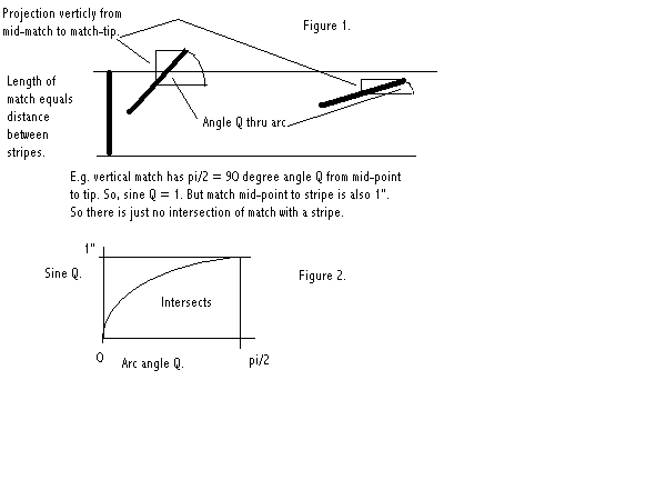
In figure 2, the X-axis gives the angle of the match with the flag's horizontal position. The Y-axis gives the sine of this angle. The match angle may vary from horizontal position, or zero degrees to the X-axis, to ninety degrees from the X-axis. That is in terms of the quadrant of a circle of possible match falls being considered. Ninety degrees has the equivalent in radians of π/2. So, the X-axis of the graph is measured from zero radians to π/2 radians.
Measuring match falls to every 15 degrees or π/12 radians, the sine length from zero angle is zero; at 15 degrees the length is .2588" or just over a quarter of an inch; at 30 degrees, the length is .5" or half an inch; at 45 degrees, the length is .707"; at 60 degrees, the length is .866"; at 75 degrees, .9659"; at ninety degrees, 1".
In other words, taking the angles at regular intervals does not result in a uniform increase in length, that would graph as a straight line sloping up-wards. Instead, a decreasing increase, in length, makes figure 2 start as a near vertical curve that increasingly turns to approach the horizontal.
If the stick falls at 30 degrees, so its sine is half an inch, then it must fall less than half an inch from a stripe to cross it. A 15 degree fall requires the stick to fall about a quarter inch or less from a stripe, to cross it. The corresponding vertical distance of about three quarters an inch, above the sine curve, at the 15 degree position on the X-axis of figure 2, belongs to the area of non-intersection (non-crossing) above the sine curve.
By the way, turning the flag stripes, from horizontal to vertical position, would simply have altered these length calculations from sines of the match's falls, to their cosines. In that case, the graph of the curve would have been reversed, starting at the one inch length, instead of the zero length. But this would have made no difference to the area of the graph under the curve.
The area of the graph under the sine curve, compared to the area of the graph over the curve, provides a probable measure of the rate of line-crossing match falls compared to within-stripe falling matches. The area under the sine curve represents all those positions, in which the distance of the match center from a line is less than the vertical distance of the match center to its head.
Therefore, comparing the under-curve area to the over-curve area gives a
probability measure of the ratio of line-crossing match falls to within-lines
match falls.
The whole area is the multiple of the Y-axis length of one inch by the X-axis
length of π/2, which gives an area of π/2 square inches.
The area under the curve can be summarily derived from the fundamental theorem of calculus that anti-differentiation gives integration, which is a summation of ever and ever smaller parts of a whole area, taken to its limit. This limit-taking of integral calculus provides the ultimate accuracy to taking successively closer approximations, with smaller rectangular steps that depart less and less from the sought area of a curve.
The differentiation of a sine produces its cosine. That means the anti-differentiation or reverse of the cosine produces the sine as its integral, or area measure.
The sine curve is considered in the range of from π/2 to zero. Subtracting the sines of these two end-values, which are one and zero, respectively, thus gives an area of one square inch under the quarter segment of the sine wave being considered.
Therefore the probable frequency of line-crossing match falls to the total of match throws is measured by the ratio of the sub-curve area of one square inch to the total area of π/2 square inches. That equals a ratio of 1/(π/2) = 2/π, which is about .636. Thus, slightly less than an average of two in every three match falls will be across stripe lines.
Now to give an electoral interpretation of the sine curve areas as a probability measure. Elections are a measure of choice and choice may be assumed to fall randomly for the candidates. Suppose no candidate is prefered to another above probable chance levels.
Also assume the scientific method of elections is the single transferable vote (STV), which uniquely for electoral systems, has similar powers of measurement, order and proportion, to the natural sciences. STV has a preference vote, giving an ordered choice of 1st, 2nd, 3rd etc candidates. This decides the order in which candidates are elected in a proportional count.
When the most prefered candidates have got more than the elective proportion, or quota, of votes in a multi-member consttituency, then surplus votes are transferable to next prefered candidates. In the interests of fairness between the voters for an elected candidate, his surplus votes are transfered according to all his voters' next preferences for different candidates. Tho, that means they all transfer a fraction, of their one vote each, that sums to the size of the surplus vote.
Very likely, the elected candidate had so many voters that he only needed a fraction of their one vote each to reach his quota. That fraction is called the keep value. The rate at which the surplus votes were transfered is called the transfer value. Every voter has one vote each, which may contribute to the election of more than one candidate. But the keep value, for the more prefered candidate, and the transfer value, for the next prefered candidate, must always add up to just one vote for every voter.
If a candidate has a keep value of one, that implies she has no more and no less than the votes needed to achieve a quota or elective proportion of the vote in a multi-member constituency. This means a zero surplus vote and so a zero transfer value to those candidate's voters' next preferences, since their votes are already used to the full without wastage or redundancy.
In scientific jargon, this rendering of equal representation might be called a conservation of votes. Of course the argument against non-transferable voting systems is that they waste votes without the information transfer of transferable voting.
The possible angles of match-stick falls, crudely measured, say every fifteen degrees, may be likened to a voter's successive orders of preference: 1st, 2nd, 3rd, 4th, 5th, 6th. The radius of one inch for the half match-stick may be likened to the one vote per voter.
Angle and radius are the forms of polar co-ordinates, as of a circle. Considering only the upper right quadrant of the circle imposed positive rectilinear co-ordinates. As the keep value and the transfer value always add up to one, the X-axis can serve as a measure of the keep value and the Y-axis as the transfer value.
The unitary radius forms the hypotenuse of a triangle with the square root of the keep value on the X-axis and the square root of the transfer value on the Y-axis as the other two sides. The square roots are in conformity with Pythagoras' theorem. At the start, the voter keeps the whole vote to herself, until she transfers it to its first and subsequent preferences to represent her.
Moving from zero degrees on the X-axis to 15 degree angle may be conventionly regarded as the voter making a first preference. The sine of 15 degrees (.2588) represents over one-quarter that voter's vote being transfered, as a result of her most prefered candidate being elected with a surplus vote.
The second prefered candidate, represented by another 15 degree turn of the radius, generates almost as great a transfer value to the vote, so that fully half that voter's vote is now transfered. The first preference kept nearly three quarters of the voter's vote to himself. The first and second preferences kept half the vote to themselves.
The successive preferences given by successive 15 degree turns generate
less and less transfers of the vote, indeed scarcely any transfer from the
fifth to the sixth preference.
This much is in accord with actual STV elections. Most of the transfers take
place between highly prefered candidates and fall off sharply towards the
lesser preferences.
From the probable decrease in voting transfers with successive transfers of the individual vote, compare the situation with the voters as a whole. An analgous condition is a probable decrease in the proportions of first preferences for successively elected candidates, by all the voters.
Assume that the individual voter in question is the average voter, whose preferences are the most typical or representative of all the voters, in that just those preferences were elected in that order by the totality of voters. Then, the average vote being less and less transferable with each succeeding preference is akin to a less and less number of first preferences given by all the voters to each successively elected candidate.
Sinusoidal probability gives an estimate of nearly 64% of the first preference votes going to elect candidates. I think I saw, once, only a slightly higher value recorded in an Irish general election. I havent been able to confirm that result. Other Irish STV election results, Ive seen, show some seventy per cent or more of first preferences are elective. That is well above my hypothesised chance level of about 64%. The 2007 Scottish local elections had nearly three-quarters of the elective votes being first preferences. And if I remember right, a lot higher levels have been recorded.
This sinusoidal model of electoral probability raises further questions. Only one quadrant of a full circle of match-falls has been interpreted electorally. What happens, when using an electoral analogy on the succeeding three quadrants?
In the second quadrant, the Y-axis of the transfer value remains the same. But the X-axis of the keep value becomes negative. Suppose the radius pointer continues from the first quadrant into the second, at 15 degree intervals. These turns may represent preferences further to, say, a first six preferences to fill a six-member constituency.
A peculiarity of the sinusoidal probability is that it is always the same, about 64%, no matter how many members in the multi-member constituency to be elected. But this situation becomes more balanced, when one considers that a second quadrant always supplies an equal number of less prefered candidates to the number to be elected.
It may be worthwhile for voters to prefer more candidates than seats, as some of their first six choices may not be elected. However, turning thru the second quadrant gradually sheds positive transfer value till a full negative keep value is achieved on the negative X-axis.
Turning thru the third quadrant, with a negative Y-axis, enables a negative keep value to be shed on negative transfer values. In other words, the third quadrant is the exact opposite of the first quadrant. Instead of being an election of candidates, it is a negative election or exclusion of candidates.
The fourth quadrant is the opposite of the second quadrant. Here one might suppose that these preferences are for the less unprefered candidates, less likely to be excluded. Eventually, the radius returns, in its counter-clock sweep, to the original positive X-axis.
The first quadrant stands for an ordinary STV election and the third quadrant may relate to some sort of anti-election or exclusion count. This is decided on the basis that in quadrant one, there is a postive keep value axis and a positive transfer value axis, where: k + t = 1. (This means that the axes themselves must be the square roots of k and t.) The third quadrant, with both axes negative, may then be symbolised: -(k + t) = 1. That is essentially the same process but negated or in reverse, as an exclusion count may be regarded with respect to an election count.
This leaves the problem of electorally interpreting the second and fourth quadrants, which may be symbolised, respectively: -k + t = 1 = -(k - t) and k - t = 1. Once again one quadrant is just the negative or reverse of the other. Bearing that in mind, both cases exhibit the phenomenum of negative transfer values, symbolised as: -t.
Traditional STV and computerised STV with Meek's method do not use negative transfer values. But I have devised, already on other web pages, a method that does, briefly explained in the next section.
I have developed a method (called Binomial STV or keep-value averaged STV, for want of a better name) with both transferably voted election and exclusion. Traditional STV's problem of "premature exclusion" means that when the surplus votes run out from the most popular candidates, the candidate who is unlucky enough to be last past the post, at that time, gets excluded, so his votes can go to help elect candidates for remaining seats.
Anyway, there is a problem with turning STV into an alternating count first of election quotas, and then when there are no more surplus votes to transfer, counting an exclusion quota. You only want to exclude one candidate, so you can re-distribute his votes again to help elect candidates in the running for remaining seats. But unless there is a quota, or more, of last preferences for a candidate, he cannot be proportionally excluded, and you are back with the corresponding problem in the exclusion count, as in the election count.
To overcome such problems, I extended the use of the rule that the keep vote plus the transfer vote must equal one vote. I did this by allowing negative transfer values. Traditional STV (including its more thoro realisation of all the permutations of transferable votes, in the computerised version called Meek's method) only uses positive transfer values, which means that the keep value never goes above one vote.
There is a good reason for this of course, the principle of one person one vote. But it is still possible to maintain this, taking into account negative transfer values and therefore keep values of greater than unity. A negative transfer value means that a candidate falls short of a quota. Taking into account negative transfer values means that the returning officer has an estimate of how much respective candidates may fall short of a quota, by how greater than unity is their keep value.
But this information is only useful if an election can be considered as
like a controled experiment or test, in which certain factors are
systematicly changed to come closer to the most consistent underlying pattern
of voting. The election is turned into a series of equitably controled
recounts. The results of the recounts are averaged for an over-all result.
In one count, a candidate may not achieve a quota, having a negative transfer
and a keep value over unity. But in another count she may over-achieve the
quota, and on average have an elective proportion of the votes, that
decisively prefers her for a seat.
This averaging of keep values, then, may sort out otherwise ambiguous results between candidates. This method, I called Binomial STV or keep value averaged STV. The reference to the binomial theorem is with regard to the binary factors of preference elections and unpreference elections or exclusions. The way these factors are combined binomially determines the system of recounts, whose keep values are to be combined and averaged. The appropriate average is the geometric mean.
Besides averages, also of importance are statistical variations about the averages. Particularly with respect to exclusion counts, one has to establish the tolerance limits by which they can be allowed to influence the outcome of the election counts. Election has primacy over exclusion, which is only resorted-to to facilitate the election. The point of an election is to elect people not exclude them.
Knowing the significance of negative transfer values offers an explanation of the second and fourth quadrants of the keep and transfer valued axes on a circle of unitary radius for one vote. The second and fourth quadrants were symbolised respectively as: -(k - t) and k - t = 1. The latter case simply applies to a candidate in an election, who has a negative transfer value, in other words, a deficit of votes from achieving a quota. He has to get his keep value down to one or below one, to be elected.
The former case is the same thing in reverse. That is for an exclusion, rather than an election. This candidate is in deficit of the votes needed to exclude her and is thus "failing" to get herself excluded, as the former candidate is failing to get himself elected.
Therefore, the electoral circle's four quadrants amount to a cycle of election and exclusion. The one-vote radius turns thru quadrant one, in discrete angles, that represent an order of preference for a given number of candidates. In the all-positive keep and transfer value quadrant, they are elected with keep values of one or less: k + t = 1.
The fourth quadrant, k - t = 1, is the other case for an election but in this case the candidates are unelected because a negative transfer value or deficit transfer value means that the keep value is correspondingly greater than one. Ive explained that an election could be held by counting the keep values of unelected candidates, by how much they are over unity, as well as by how much elected candidates have keep values less than unity.
As a supplement to this, a negative election or exclusion could be held, as symbolised by the other two quadrants. The third quadrant, symbolised by -(k + t) = 1, is just like an election transfer of surplus votes to next prefered candidates, except that it is now an exclusion transfer of surplus votes to the next least prefered candidates.
The second quadrant, -(k - t) = 1, covers those candidates, in an exclusion count, who have keep values over unity. Unity keep value is the quota level of votes, they have not got down-to, to get themselves excluded. Their negative or deficient transfer values means they are not unprefered or unpopular enough to pass their unpopularity onto next less prefered candidates.
Dividing the probability circle verticly in half gives an election hemisphere, on the right, and an exclusion hemisphere, on the left. The principle of one person one vote, in an election, may be symbolised by multiplying: (k + t)(k - t) = 1. And similarly for the exclusion hemisphere.
One complete turn of a circle corresponds to a rectilinear graph of one complete sine wave, crest and trof. If the circle is turned ninety degrees, so the election hemisphere is on top, then it would correspond to the crest of the wave, with the exclusion hemisphere as the trof.
The circle might go thru many turns and the wave repeat itself as many times. This might be envisioned as many elections, or polls with both election and exclusion counts, in which definite representation is reached after many "waves" of candidates have been successively elected and excluded, something in the manner of primaries. Alternatively, the many waves could be stretched not over time but over space, in many constituencies, like a general election.
My example of a binomial STV election of the first degree corresponds to the situations covered by the two hemispheres of the probability circle. STV, first degree, consists of an election for the keep values of the candidates, whether or not they achieve out-right election, and an exclusion of those candidates whether or not they achieve out-right exclusion. The exclusion keep values are inverted to turn relative unpopularity into a second estimate of relative popularity.
The election keep values and the inverted exclusion keep values are then averaged (with the geometric mean) for a most typical keep value per candidate. As for all the statistics of representation, there is no absolutely right answer. The closer the contest, the more the out-come must rely on probability estimates of who exactly are the most prefered candidates.
However, in most elections, there is not much doubt about who are the most
prefered. And where there is genuine doubt, it may be safely said that a
challenge to the result, within statistical margins for disagreement, has low
legitimacy. Indeed, it is vital, given the truly statistical nature of
electoral representation, that contestants agree beforehand on the
statistical margins they will work with, in determining the result.
With Binomial STV, this chiefly means deciding within what statistical
margins to allow an exclusion count to weigh with an election count, that
may, on occasion, be otherwise ambiguous, usually in the late stages of the
count.
Such considerations of establishing confidence limits, within which to assess results, are universal to statistics. And there is no reason why they cannot be applied objectively to electoral procedure. The only objection can be the low level of objectivity, to which we are accustomed, in politics. Professional standards of honesty, by which the natural sciences have achieved so much, would be required.
In the previous section, negative transfer values were considered from my keep-value averaged STV method. These transfer values are in deficit of the votes needed by a candidate to achieve a quota, rather than the surplus votes a candidate may have over a quota.
It is possible to re-state positive or surplus transfer values, where k + t = 1, and negative or deficit transfer values, where k - t = 1, in terms of imaginary transfer values. The imaginary number, i, equals the square root of minus one. Then, if T = it, k + t = k - i.it = k - iT.
And k - t = k + i.it = k + iT.
Imaginary numbers are basic to modern mathematics and prevail thru much of natural science. Historicly, they were more of a mystery than they are now, and the name, imaginary number, as distinct from "real" number, has stuck. Ive used them on my pages about Minkowski's Interval in Special Relativity. That is to say where different observerrs allow for their relative motions in measuring an event somewhat approaching light speed. There, the velocities of the observers or of light itself are commonly expressed as imaginary numbers.
On my page claiming that Minkowski's Interval predicts the Michelson-Morley experiment, I introduced the notion that an imaginary velocity refered to the transverse motion of light with respect to the earth, as distinct from the longitudinal motion of light aligned with the earth's motion. In other words, the "imaginary" velocity is just an out-dated term that actually shows motion at right angles to the so-called "real" motion.
This reference to the Interval is just to show that an imaginary number usually refers to a dimension at right angles to a real number dimension. With respect to transfer values, conventional transferable voting method only knows positive transfer values. I introduced negative transfer values for a new STV method. That gives both a positive and a negative axis of transfer values, which are at 180 degrees to each other, in Cartesian co-ordinates.
This leads to the question: what signifies an imaginary axis of transfer values, at ninety degrees to the positive and negative axes? Well, if you look at the traditional voting practise in assemblies, there are three common responses to an issue. Members vote for it, they vote against it, or they abstain. So, there are positive votes, negative votes, and neutral votes.
Neutral votes seem to fit the bill as to what are imaginary votes. They
come in between outright Yes and No votes, existing in a dimension of their
own. Neutrality should not be confused with other things. It is not a refusal
to vote at all. It is merely an assertion that on some issue the voter is not
aligned for or against.
Neutral votes could be valuable to express tolerance. That is against making
an issue, for or against things, that you would rather were left alone.
Neutral votes might serve as a protest or veto against too much law-making
and intrusion by law-makers in matters that do not concern them.
Nor should neutrality be confused with the option, None of the above. NOTA is a rejection of all the candidates standing in an election. It is an out-right exclusion, in the hope of another election with acceptable candidates.
Preference voting implies either a positive or negative order of choice of candidates (or issues). It is questionable whether a neutral vote or abstention can order candidates or issues by how neutral one feels towards them. Still, it may be possible to have a scale consisting of degrees of neutrality as unwillingness to vote for or against given policies or politicians.
It might seem more logical to treat a neutral scale as a random order of choice. But this cannot necessarily be assumed. The attempt to set out an order of unwillingness is subject to test as to its randomness. For, neutrality on a given range of issues or candidates might, or might not, mean that the voters, as a whole, show over-all unwillingness towards them.
This page originally suggested sinusoidal probability as a test of whether first preferences played a bigger part in electing candidates than expected from a random order of choice between the candidates.
Probability theory traditionly treats probabilities as solely positive.
The form, it is put in, is that the chance of an event occuring, its
"success", p, plus the chance of its not occuring, its "failure", q, is equal
to unity: p + q = 1.
This is analgous to the definition of keep values, k, and transfer values, t,
in traditional STV: they both are positive fractions that add up to unity.
The election means a choice but a choice can be measured in terms of how much
a chance result it appears to be, in terms of how much the elected candidates
are favored over the unelected.
My new STV electoral methods use more voting information, than traditional
methods, by involving negative transfer values, whereby k - t = 1.
Analgously, negative probability can be conceived such that p - q = 1.
Moreover, from discussing the possibility of imaginary transfer values, in
abstentions, imaginary probabilities are also conceivable, of the form, say:
p - q = p + iQ.
The circle of probability seems to match first order Binomial STV. There
is an election using keep values with negative as well as positive transfer
values. And this is averaged with a reverse-preferenced election, as an
exclusion, subject to conventionly agreed limits of tolerance, especially as
to the latter's validity.
The first order Binomial STV consists of two counts: one election qualified
by one exclusion, or a preference count and an unpreference count.
(Traditional STV is zero order Binomial STV, where the election is
unqualified by an exclusion - or vice versa.)
My pages also give examples of second-order Binomial STV, which consists not of just two counts but of four counts, differently qualified by combinations of preference and unpreference, according to a (non-commutative) expansion of the binomial theorem (to the power of two) in binary terms of preference and unpreference.
Such complicating refinements are unlikely to be needed in ordinary elections, and, I would guess from the few examples I tried by hand count, almost certainly not beyond the second order Binomial STV. Certainly the future of STV is with computerised counts. But there is also a case for studying the trade-off between efficiency and simplicity in STV counts.
And it is a point about simplicity that concerns this section. I suggested that first order Binomial STV corresponds to a circle of preference and unpreference. This itself corresponds to a graph of sinusoidal probability, that enabled me to hazard an approximate 64% of votes, that elect candidates as first preferences, probabiy not shown undue preference.
However, I would suggest that second order Binomial STV and higher orders could not be expressed in terms of a circle generating a sine wave. On my page that draws a graph of the Fibonacci series, one has the x-ordinate start from the first term, say zero, and the y-ordinate start from the second term, one, in the series.
The Fibonacci series is algorithm based on the ordered numbers, 1, 2, 3, 4,.. But this simple arithmetic series is not itself elementary. It already has been created out of simple algorithm. This operation is evident in the outer flanks of Pascal's triangle, which consists of diagonals of ones. These cumulatively add down the rows, in effect defining 1, 2, 3, etc as successive additions of one.
I mention this, because it is much more obvious that the binomial series is already a structured number system before applying further operations on it. But that doesnt make algorithm on the binomial series in principle any different from the Fibonacci series as algorithm on the basic arithmetic series, known as the "natural" number system.
The Binomial series can be subject to different algorithmic options. The way, most like the Fibonacci series graph as an angular damped wave, gives higher order binomial expansions as approximations, from a discrete wave consisting of straight lines joined at angles, ever closer towards a continuous curve.
Algorithm for discrete (undamped) waves using orders of binomial series, as in the successive rows of Pascal's triangle, can be as follows. Taking the first row of Pascal's triangle (010) this is rendered into x-y co-ordinate pairs: 01, 10. Repeat these two co-ordinates in reverse: 10, 01. Then add the whole series cumulatively: 01, 11, 21, 22. Starting from the origin, 00, this series gives a simple zig-zag wave with angle crest and angle trof, whose equilibrium is a forty-five degree line between between the x and y axes. The wave can be continued indefinitely by continuing above algorithm.
This is similar to the Fibonacci series wave, which is also a zig-zag, except that it is damped or the wave rapidly subsides to the equilibrium line, which is at a steeper angle than forty-five degrees.
It was discovered sometime late in the nineteenth century, that the Fibonacci series can be derived from Pascal's triangle. Instead of looking at the level rows, you put a series of parallel slanting lines thru Pascal's triangle. Sum each successive slanted row and it gives the successive terms of the Fibonacci series. These slant sums are: 0, 0 +1, 0 + 1, 0 + 1 + 1 = 2, 0 + 1 + 2 = 3, 0 + 1 + 3 + 1 = 5,..
These Fibonacci-Pascal rows can also be given the treatment for Pascal rows, so that they can be graphed as waves, except that their tendency is to break out of the wave shape into one-sided crests of indefinite height.
This is distinct from skewed forms of the binomial series, where both terms in the factor of the binomial theorem are not equal. Pascal's triangle gives the symetrical form resulting from equal terms. For example, instead of two terms both of one-half, the two terms might be three-quarters and one quarter. Expanding these terms by raising their factor to some power results in a skewed or asymetrical distribution. This, too, with above algorithm results in waves but skewed waves instead of symetrical waves.
In both the symetrical and skewed versions, an example was chosen that summed to unity. If unity stands for the sum of probabilities, then the differing wave forms' areas between the wave crest and equilibrium line, might graphicly represent kinds of probability distribution. To borrow the quantum physicists' term, they might be considered as kinds of "probability waves."
Exactly the same procedure can be followed for succeeding rows of Pascal's triangle, as was followed for the first line, 010. The next row is: 0110. It graphs not as a zig-zag or single poled tent shape crest but with a crest like a twin-topped tent, and a similarly shaped trof, like a zinc bath-tub.
Mathematicians first tried to understand wave motion using such simplified wave shapes. Angular waves like this could be made by putting two small weights at distances along a vibrating string. (I discuss this on my page: Coupled oscillator and wave equation.)
Higher powers of the binomial theorem, squared, cubed, etc graph more angles in the "wave," which (when reduced in scale) look more like continuous curves of a real flowing wave. But, as the term binomial implies, only two dimensions are considered.
Using algorithm, as before, on the trinomial theorem produces discrete waves in three dimensions. That is spirals. If, like me, you are unfamiliar with 3-D computer software (which I believe uses projective geometry to create perspectives) you can still use the old-fashioned cartography to graph a spiral from the trinomial theorem. Not to any sophistication, of course - computers are essential for that - but just to show it works.
For example, suppose that the probability is equal that one moves in any of three dimensions of space. That is probabilities of one-third each for moving back and forth or up and down or left and right. The factor (1/3 + 1/3 + 1/3) can be expanded by successive powers of zero, one, two, etc...
Take the power of one, which is simply the above factor. Factor out the common denominator of 3, and put zeros on either side of the three ones (also implicit in Pascal's triangle). Then the full first order trinomial series row is: 01110. This row is put into triplets, representing co-ordinates in three dimensions. Thus: 011, 111, 110, then in reverse: 110, 111, 011. Cumulate the whole series for: 011, 122, 232, 342, 453, 464. These may be considered respectively as the x,y,z co-ordinates.
Draw a plan graph of the x and y co-ordinates. Join up the points, starting from the origin, 00. Then the z ordinate may be considered the height of each plotted x,y position, and marked beside each co-ordinate, as heights are given on a contour map. Even tho this is only the very first order expansion of the trinomial theorem, a very crude spiral can be discerned from its mapping.
One doesnt have to stop with the trinomial theorem. One could build a three-dimensional spiral model and mark its co-ordinates with four-dimensional indicators. Beyond model-making, hyper-dimensional wave forms can still be created from applying afore-said algorithm to the multinomial theorem.
A variation, on algorithm for graphing the binomial series, can be given here. Pascal's triangle row, 010, is succeeded by 0110. Let the matching x and y co-ordinates be as in table 1.
| X | Y |
| 0 | 1 |
| 1 | 1 |
| 1 | 0 |
Drawing a graph of table 1, starting at the x-y origin of 0,0, generates a square. But it becomes apparent from similarly graphing successive rows of Pascal's triangle that the square approximates a circle.
(The formulas for a circle also suggest this relation to the square. The area of a circle, πr², suggests a square (whose sides are the radius of a corresponding circle) multiplied by a constant of curvature, π, equal to a circle hemisphere divided by its radius.)
Graphing the second order binomial series (expanding the binary terms to
the power of two) produces a water-drop shape like some of the so-called
standard polar curves. A tear shape is but a circular drop pulled out by
gravity.
The higher the order of expansion the more out of shape the original circle
becomes, the more extended the tear-drop, like from a leaking tap, only
indefinitely so.
A circle is a symetrical shape that generates the symetrical wave of a sine curve. But a tear shape has no such obvious locus, as a wheel has a hub, to generate a correspondingly simple wave pattern, to use as a probability measure.
The first order expansion (to the power of one) corresponds to first order
STV and graphing it produces a circle, with the binomial terms of preference
and unpreference.
Ordinary numbers, say, the two number ones in the first order row of Pascal's
triangle, are commutative. But the terms p and u are terms of logical
procedure in my Binomial STV counts, and so the expansion of the binomial
theorem for p and u, is non-commutative.
Whichever algorithm used on Pascal's triangle rows, the one for waves or the one for drops, the first order row implies a circle, for my purposes, of preference and unpreference or election and exclusion. And the circle generates a sinusoidal "probability wave."
Perfect numbers are those whose divisors add up to the number itself. For example 6 is dividable by 1, 2 and 3, which sum to 6. Perfect numbers are also the sum of a series of consecutive counting numbers.
Pythagoras, who studied perfect numbers, also discovered they were closely linked to twoness. He discovered that powers of two have divisors that always add up to just one less. So, 2^2 = 4 is divisible by 1 and 2, which add to three; 2^3 = 8 is divisible by 1, 2, 4, which add to 7.
Of the shortfall of one, Simon Singh's book on Fermat's Last Theorem, says
"This makes them only slightly defective."
But I'd like to point out, that if you extend consideration of powers of two
from positive powers to negative powers, then they are not even slightly
defective perfect numbers.
Table 2 shows that the shortfall of one is made good by the divisors of the negative powers of two. These form an infinite sum, which converges to one.
| Powers of two. | Divisors. |
| 2^-4 = 1/16 | 1/32, 1/64, 1/128,.. |
| 2^-3 = 1/8 | 1/16, 1/32, 1/64,.. |
| 2^-2 = 1/4 | 1/8, 1/16, 1/32,.. |
| 2^-1 = 1/2 | 1/4, 1/8, 1/16,.. |
| 2^0 = 1 | 1/2, 1/4, 1/8,.. |
| 2^1 = 2 | 1, 1/2, 1/4, 1/8,.. |
| 2^2 = 4 | 2, 1, 1/2, 1/4,.. |
| 2^3 = 8 | 4, 2, 1, 1/2, 1/4,.. |
| 2^4 = 16 | 8, 4, 2, 1, 1/2, 1/4,.. |
Sometimes the convergence to one is shown by the picture of a square of one unit by one unit or one square unit. Firstly the square is divided in half, then the other half is itself divided in half. This means that the first two terms, 1/2 and 1/4, already cover three-quarters of the unitary square. The third term, 1/8, takes away one half of the remaining quarter, leaving just an eighth of the square uncovered. In fact, every successive term, which is half the size of the preceding term, leaves only the same size as itself uncovered. Thus the series continues indefinitely to converge to unity.
Taking this into account these slightly defective perfect squares are better called infinitely perfect squares, because in taking the series of positive and negative powers of two to an infinite limit, they become perfect numbers.
Simon Singh says since Pythagoras' time mathematicians are still unable to prove whether no slightly "excessive numbers" exist. That is numbers whose divisors add to just over that number. But it is apparent that if "slightly defective" numbers is a misleading way to look at them, then the notion of slightly excessive numbers is also misleading. In other words, the inability to find the right answer owes to the wrong question.
The conception of infinitely perfect numbers has a useful application as a formula for the generation of successive rows of Pascal's triangle. For any given row, say the nth row, given by the binomial theorem: (a + b)^n, where a = b = 1, this is given by the sum of all the previous rows from the power of minus infinity to the power of n minus one.
My page, The diffusion equation as a finite difference equation, is about this generation of Pascal's triangle over time. The equation consists of a dependent variable of concentration that is subject to two independent variables in space and over time, in which a diffusion occurs. This can mean the conduction of heat, or diffusion of molecular agitation both ways from the heated center of a metal bar, when considering diffusion in approximately only one dimension.
In the classical calculus of continuous motion, the diffusion equation is of a second order spatial term to a first order temporal term. The infinitely perfect numbers conception provides a discrete formula analgous to the classical temporal term. It is just a discrete formula for the "diffusion" of Pascal's triangle, each row succeeded by a wider row.
Whereas the spatial term is equivalent to the well-known binomial theorem for any given row of Pascal's triangle. The number of the row is matchable to the number of the power used to expand the binomial theorem into a binomial series, which is what a row of Pascal's triangle is.
Linking the binomial theorem to an infinitely perfect numbers conception, thus gives an algebraic version of the classical diffusion equation.
References.
George Gamov: One, Two, Three...Infinity.
Simon Singh: Fermat's Last Theorem.
Martin Gardner: Mathematical Carnival.
Richard Lung.
23 February 2009.